DNN with backpropagation in C++, part 2
Two layer NN with backpropagation in C++
Now let’s implement a two layer neural-network in C++.
As a staring point we’ll use source code from “DNN with backpropagation in C++”, part 1
Again, to keep it simple we’ll assume:
- there’s no bias in the dense layers;
- there’s no non-linear activation;
- loss function is Mean Squared Error.
Forward path for input vector X of size M, and 2 layer neural net with \(M\) inputs and \(N\) outputs
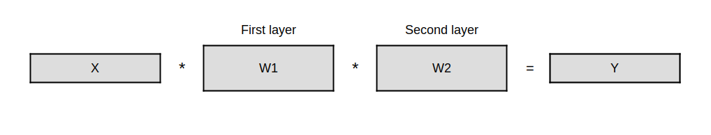
Two layer neural net output \(Y\) is:
\[Y_{1} = X * W_{1}\] \[\hat Y = Y_{1} * W_{2}\]where
\(X\) is input vector
\(W_{1}\) are weights for dense layer 1
\(Y_{1}\) is output of dense layer 1
\(W_{2}\) are weights for dense layer 2
\(Y\) is expected (true) output of neural net:
\[Y = \left( \begin{array}{ccc} y_{0} & y_{1} & \ldots & y_{N-1} \\ \end{array} \right)\]\(\hat Y\) is predicted output vector:
\[\hat Y = \left( \begin{array}{ccc} \hat y_{0} & \hat y_{1} & \ldots & \hat y_{N-1} \\ \end{array} \right)\]Mean Squared Error (MSE) loss between predicted \(\hat Y\) and expected \(Y\) is
\[E = MSE(Y, \hat Y) = \frac {1} {N} \sum_{i=0}^{N-1} ( Y_{i} - \hat Y_{i} )^2\]Error backpropagation.
For input \(X\), we want to minimize the MSE difference between out network output and expected output, by adjusting weights of both dense layers:
\[\frac {\partial E} {\partial W_{1}}\] \[\frac {\partial E} {\partial W_{2}}\]Adjustment for dense layer 2 weights is going to be the same as in the previous post “Dense layer with backpropagation in C++”
Let’s find weight adjustment for the weights of dense layer 1.
\[\hat Y = X * W_{1} * W_{2}\]Using chain rule
\[\frac {\partial E} {\partial W_{1}} = \frac {\partial E} {\partial \hat Y} * \frac {\partial \hat Y} {\partial W_{1}}\]or
\[\frac {\partial E} {\partial W_{1}} = \frac {\partial E} {\partial \hat Y} * \frac {\partial \hat Y} {\partial Y_{1}} * \frac {\partial Y_{1}} {\partial W_{1}}\]where
\[\frac {\partial E} {\partial \hat Y} = \frac {2 * ( \hat Y - {Y} )} {N}\] \[\frac {\partial \hat Y} {\partial Y_{1}} = W_{2}^T\] \[\frac {\partial Y_{1}} {\partial W_{1}} = X^T\]Finally, the weight updates are:
\[\frac {\partial E} {\partial W_{1}} = \frac {2 * ( \hat Y - {Y} )} {N} * W_{2}^T * X^T\]First, let’s write Python implementation with TF2. We’ll use it to validate C++ code in the consecutive section.
For this experiment I’ve used the following software versions:
$ python3 -m pip freeze | grep "numpy\|tensorflow"
numpy==1.19.5
tensorflow==2.5.0rc2

$ g++ --version
g++ 9.3.0
Python code will be very similar to Python sample from the prevoius post.
Import TF and Keras. We’ll define a network with 2 inputs and 2 outpus.
import tensorflow as tf
from tensorflow.keras.layers import Dense
from tensorflow.keras.optimizers import RMSprop
import numpy as np

num_inputs = 2
num_outputs = 2
# Create two layer model
model = tf.keras.Sequential()
# No bias, no activation, initialize weights with 1.0
layer1 = Dense(units=num_inputs, use_bias=False, activation=None, kernel_initializer=tf.keras.initializers.ones())
layer2 = Dense(units=num_outputs, use_bias=False, activation=None, kernel_initializer=tf.keras.initializers.ones())
model.add(layer1)
model.add(layer2)Use mean square error for the loss function.
# use MSE as loss function
loss_fn = tf.keras.losses.MeanSquaredError()
Hardcode model input and expected model output. We’ll use the same array values later in C++ implementation.
# Arbitrary model input
x = np.array([2.0, 0.5])

# Expected output
y_true = np.array([2.0, 1.0])
Use Stochastic Gradient Decent (SGD) optimizer.
SGD weight update rule is \(W = W - LR * \nabla\)
\(\nabla\) is weight gradient and \(LR\) is learning rate.
For now we’ll assume learning rate equal to 1.0
# SGD update rule for parameter w with gradient g when momentum is 0 is as follows:
#   w = w - learning_rate * g
#
#   For simplicity make learning_rate=1.0
optimizer = tf.keras.optimizers.SGD(learning_rate=1.0, momentum=0.0)
In the training loop we’ll compute model output for input X, compute and backpropagate the loss.
# Get model output y for input x, compute loss, and record gradients
with tf.GradientTape(persistent=True) as tape:

    # get model output y for input x
    # add newaxis for batch size of 1
    xt = tf.convert_to_tensor(x[np.newaxis, ...])
    tape.watch(xt)
    y = model(xt)

    # loss gradient with respect to loss input y
    dy_dw = tape.gradient(y, model.trainable_variables)

    # obtain MSE loss
    loss = loss_fn(y_true, y)

    # loss gradient with respect to loss input y
    dloss_dy = tape.gradient(loss, y)

    # adjust Dense layer weights
    grad = tape.gradient(loss, model.trainable_variables)
    optimizer.apply_gradients(zip(grad, model.trainable_variables))
Finally we’ll print inputs, outputs, gradients, and updated Dense layer weights.
# print model input and output excluding batch dimention
print(f"input x={x}")
print(f"output y={y[0]}")
print(f"expected output y_true={y_true}")

# print MSE loss
print(f"loss={loss}")

# print loss gradients
print("dloss_dy={}".format(*[v.numpy() for v in dloss_dy]))

# print weight gradients d_loss/d_w
print("grad=\n{}".format(*[v.numpy() for v in grad]))

# print updated dense layer weights
print("updated weights=")
print(*[v.numpy() for v in model.trainable_variables], sep="\n")
After running Python example we get:
$ python3 dense2.py
input x=[2.  0.5]
output y=[5. 5.]
expected output y_true=[2. 1.]
loss=12.5
dloss_dy=[3. 4.]
grad=
[[14.  14. ]
 [ 3.5  3.5]]
updated weights=
[[-13.  -13. ]
 [ -2.5  -2.5]]
[[-6.5 -9. ]
 [-6.5 -9. ]]
Let’s code the same example in C++
in C++ implementation we’ll compute
\[\frac {2 * ( Y - \hat {Y} )} {N} * W_{2}^T\]as output of backward() function of the dense layer.
This will allow us to feed backward() output of a layer as input to backward() function for the previous layer.
We’ll implement it using C++ STL. Chrono headers are included for clocks used to benchmark run time.
#include <cstdio>
#include <vector>
#include <algorithm>
#include <cassert>
#include <numeric>
#include <array>
#include <chrono>
#include <iostream>
#include <string>
#include <functional>
#include <array>
#include <iterator>

using namespace std;
using std::chrono::high_resolution_clock;
using std::chrono::duration_cast;
using std::chrono::microseconds;
Lambda will be used to pretty print inputs, outputs, and layer weights.
/*
 * Print helper function
 */
auto print_fn = [](const float& x)  -> void {printf("%.1f ", x);};
Dense layer weights initializer.
/*
 * Constant 1.0 weight intializer
 */
static auto ones_initializer = []() -> float
{
  return 1.0;
};
Dense layer class template includes forward() and backward() functions. Backward() function was modified from the previous example to return backpropagated gradient.
/*
 * Dense layer class template
 *
 * Parameters:
 *  num_inputs: number of inputs to Dense layer
 *  num_outputs: number of Dense layer outputs
 *  T: input, output, and weights type in the dense layer
 *  initializer: weights initializer function
 */
template<size_t num_inputs, size_t num_outputs, typename T = float,
         T (*initializer)()=ones_initializer>
struct Dense
{

  typedef array<T, num_inputs> input_vector;
  typedef array<T, num_outputs> output_vector;

  vector<input_vector> weights;

  /*
   * Dense layer constructor
   */
  Dense()
  {
    /*
     * Create num_outputs x num_inputs matric
     */
    weights.resize(num_outputs);
    for (input_vector& w: weights)
      {
        generate(w.begin(), w.end(), *initializer);
      }
  }

  /*
   * Dense layer backward pass
   */
  input_vector backward(input_vector& input, output_vector dloss_dy)
  {
    /*
     * Weight update according to SGD algorithm with momentum = 0.0 is:
     *  w = w - learning_rate * d_loss/dw
     *
     * For simplicity assume learning_rate = 1.0
     *
     * d_loss/dw = dloss/dy * dy/dw
     *
     * dy/dw is :
     *  y = w[0]*x[0] + w[1] * x[1] +... + w[n] * x[n]
     *  dy/dw[i] = x[i]
     *
     * For clarity we:
     *  assume learning_rate = 1.0
     *  first compute dw
     *  second update weights by subtracting dw
     */

    /*
     * compute dw
     * dw = outer(x, de_dy)
     */
    vector<input_vector> dw;
    for (auto dloss_dy_i: dloss_dy)
      {
        auto row = input;
        for_each(row.begin(), row.end(), [dloss_dy_i](T &xi){ xi *= dloss_dy_i;});
        dw.push_back(row);
      }

    /*
     * Compute backpropagated gradient
     */
    input_vector ret;
    transform(weights.begin(), weights.end(), ret.begin(),
              [dloss_dy](input_vector& w)
              {
                T val = inner_product(w.begin(), w.end(), dloss_dy.begin(), 0.0);
                return val;
              });

    /*
     * compute w = w - dw
     * assume learning rate = 1.0
     */
    transform(weights.begin(), weights.end(), dw.begin(), weights.begin(),
              [](input_vector& left, input_vector& right)
              {
                transform(left.begin(), left.end(), right.begin(),
                          left.begin(), minus<T>());
                return left;
              });

    return ret;
  }

  /*
   * Helper function to convert Dense layer to string
   * Used for printing the layer
   */
  operator std::string() const
  {
    std::ostringstream ret;
    ret.precision(1);

    for (int y=0; y < weights[0].size(); y++)
      {
        for (int x=0; x < weights.size(); x++)
          {
            if (weights[x][y] >= 0)
              ret << " ";
            ret << std::fixed << weights[x][y] << " ";
          }
        ret << std::endl;
      }
    return ret.str();
  }

  /*
   * Helper function to cout Dense layer object
   */
  friend ostream& operator<<(ostream& os, const Dense& dense)
  {
    os << (string)dense;
    return os;
  }

};
Mean Squared Error class is the same s in the previous post
/*
 * Mean Squared Error loss class
 * Parameters:
 *  num_inputs: number of inputs to MSE function.
 *  T: input type, float by defaut.
 */
template<size_t num_inputs, typename T = float>
struct MSE
{
  /*
   * Forward pass computes MSE loss for inputs y (label) and yhat (predicted)
   */
  static T forward(const array<T, num_inputs>& y, const array<T, num_inputs>& yhat)
  {
    T loss = transform_reduce(y.begin(), y.end(), yhat.begin(), 0.0, plus<T>(),
                              [](const T& left, const T& right)
                              {
                                return (left - right) * (left - right);
                              }
                              );
    return loss / num_inputs;
  }

  /*
   * Backward pass computes dloss/dy for inputs y (label) and yhat (predicted)
   *
   * loss = sum((yhat[i] - y[i])^2) / N
   *   i=0...N-1
   *   where N is number of inputs
   *
   * d_loss/dy[i] = 2 * (yhat[i] - y[i]) * (-1) / N
   * d_loss/dy[i] = 2 * (y[i] - yhat[i]) / N
   *
   */
  static array<T, num_inputs> backward(const array<T, num_inputs>& y,
                                       const array<T, num_inputs>& yhat)
  {
    array<T, num_inputs> de_dy;

    transform(y.begin(), y.end(), yhat.begin(), de_dy.begin(),
              [](const T& left, const T& right)
              {
                return 2 * (right - left) / num_inputs;
              }
              );
    return de_dy;
  }

};
Finally, in the main function, we’ll declare input x and expecetd output y_true arrays, containing the same values as in out Python example. Then we’ll compute forward and backward passes, and print the network output and updated weights.
int main(void)
{
  const int num_inputs = 2;
  const int num_outputs = 2;
  const int num_iterations = 1000;

  array<float, num_inputs> x = {2.0, 0.5};
  array<float, num_outputs> ytrue = {2.0, 1.0};

  /*
   * Create dense layer and MSE loss
   */
  Dense<num_inputs, num_outputs> dense1;
  Dense<num_inputs, num_outputs> dense2;
  MSE<num_outputs> mse_loss;

  /*
   * Compute Dense layer output y for input x
   */
  auto y1 = dense1.forward(x);
  auto y2 = dense2.forward(y1);

  /*
   * Copute MSE loss for output y and labe yhat
   */
  auto loss = mse_loss.forward(ytrue, y2);

  /*
   * Benchmark Dense layer inference latency
   */
  auto ts = high_resolution_clock::now();
  for (auto iter = 0;  iter < num_iterations; iter++)
    {
      y1 = dense1.forward(x);
      y2  = dense2.forward(y1);
    }
  auto te = high_resolution_clock::now();
  auto dt_us = (float)duration_cast<microseconds>(te - ts).count() / num_iterations;

  /*
   * Print DNN input x
   */
  printf("input x=");
  for_each(x.begin(), x.end(), print_fn);
  printf("\n");

  /*
   * Print DNN output y
   */
  printf("output y1=");
  for_each(y1.begin(), y1.end(), print_fn);
  printf("\n");

  printf("output y2=");
  for_each(y2.begin(), y2.end(), print_fn);
  printf("\n");

  /*
   * Print loss for output y and label ytrue
   */
  printf("loss: %f\n", loss);

  /*
   * Compute dloss/dy gradients
   */
  auto dloss_dy = mse_loss.backward(ytrue, y2);

  /*
   * Back propagate loss
   */
  auto bw2 = dense2.backward(y1, dloss_dy);
  dense1.backward(x, bw2);

  /*
   * print dloss/dy
   */
  printf("d(loss)/dy: ");
  for_each(dloss_dy.begin(), dloss_dy.end(), print_fn);
  printf("\n");

  /*
   * Print updated Dense layer weights
   */
  printf("updated dense 1 layer weights:\n%s", ((string)dense1).c_str());
  printf("updated dense 2 layer weights:\n%s", ((string)dense2).c_str());

  /*
   * Print average latency
   */
  printf("time dt=%f usec\n", dt_us);

  return 0;
}
After compiling and running C++ example we get:
$ g++ -o dense2 -std=c++2a dense2.cpp && ./dense2
input x=2.0 0.5
output y1=2.5 2.5
output y2=5.0 5.0
loss: 12.500000
d(loss)/dy: 3.0 4.0
updated dense 1 layer weights:
-13.0 -13.0
-2.5 -2.5
updated dense 2 layer weights:
-6.5 -9.0
-6.5 -9.0
time dt=0.187000 usec
As one can verify, forward path output of the C++ implementation matches the Python code. Also, gradients and Dense layer weights after backpropagation match in Python and C++ code.
Python source code for this example is at dense2.py
C++ implementation is at dense2.cpp