Gumbel Softmax

Gumbel-Softmax

In some deep learning problems we need to draw samples from a categorical distribution.

For example, in certain reinforcement learning algorithms, next action is sampled randomly from probabilities $\pi$ predicted by policy DNN

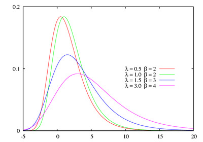
\[z = argmax(G + log(\pi))\]

Where $\pi$ are action probabilities and $G$ is random value with Gumbel distribution defined by PDF

\[f(x) = \frac {1} {\beta} e^{\frac {x-\lambda} {\beta} } e^{-e^{\frac {x-\lambda} {\beta}}}\]

Gumbel PDF

gumbelpdf

where $\lambda$ is location and $\beta$ is scale parameters.

The case where $\lambda = 0$ and $\beta = 1$ is called the standard gumbel distribution with PDF:

\[f(x) = e^x e^{-e^x}\]

We can’t backpropagate the error through argmax layer because argmax function is not differentiable.

Argmax can be approximated with a differentiable Softmax function, allowing to sample discrete random values in a differentiable way.

Softmax $\sigma(x)$:

\[z = \sigma \left(G + log(\pi) \right)\] \[\sigma {(\boldsymbol{x}_{i})} = \frac {e^{\frac {x_{i}} {\tau}}} {\sum_{i=1}^{M} e^{ \frac {x_{i}} {\tau}}}\]

Where ${\tau}$ is Softmax temperature. Temperature ${\tau}$ is a hyperparameter, changing softmax probabilities: lower temperatures make softmax output probabilities more “confident”. Taking $\lim\limits_{\tau \to 0}$, softmax $\sigma(x, \tau)$ will produce one-hot vector.

Using gumbel softmax let’s implement differentiable layer for finding index of the largest value in the input random array.

Numpy implementation:

import numpy as np

# generate array
max_value = 5
x = np.arange(max_value).astype(np.float32)
np.random.shuffle(x)

# find and print index of the largest value
max_index = np.argmax(x)
print(f"x={x} max_index={max_index}")

$ python3 test.py
x=[3. 1. 0. 4. 2.] max_index=3

As expected, the largest value in the input array [3, 1., 0., 4., 2.] is at index 3

Now let’s use a DNN to solve the same problem. First, similar to the python code, we’ll use Tensorflow argmax wrapped in a custom Sample_Argmax layer.

import tensorflow as tf
from tensorflow.keras.layers import Dense, Layer
from tensorflow.keras.optimizers import RMSprop
from tensorflow.keras import backend as K
import numpy as np

# number of integers in the input array
num_values = 5

# Custom layer to return index of distribution sample
class Sample_Argmax(Layer):

    def __init__(self, num_values=5):
        super(Sample_Argmax, self).__init__()

    def call(self, dist):
        noise = np.random.gumbel(size=x.shape)
        noisy_x = dist + noise
        return K.argmax(noisy_x, axis=-1)

# toy model with one Dense layer and one custom sample layer
model = tf.keras.Sequential()
model.add(Dense(num_values, activation=None, use_bias=False,
                kernel_initializer=tf.keras.initializers.zeros()))
model.add(Sample_Argmax())

# loss function is L1 distance between predicted and actual indexes
def loss_fn(target, x_pred):
    x_pred = tf.cast(x=x_pred, dtype=tf.float32)
    return tf.math.reduce_sum(tf.math.abs(x_pred - target))

# Optimizer with 0.5 learning rate
optimizer=RMSprop(lr=0.5)

# Traininig input is shuffled array of integers
x = np.arange(num_values).astype(np.float32)
np.random.shuffle(x)

# and label is index of the maximum value in the array
y = np.argmax(x)

# Training loop
for idx in range(3):
    with tf.GradientTape() as tape:
        pred = model(x[np.newaxis, ...])
        pred = pred[0]
        loss = loss_fn(y, pred)
        grad = tape.gradient(loss, model.trainable_variables)
    optimizer.apply_gradients(zip(grad, model.trainable_variables))
    print(f"Training x={x} tgt={y} pred={pred:.1f)} loss={loss:.2f}")

# Test
pred = model(x)[0]
print(f"Testing x={x} expected y={y} pred={pred:.1f}")

$ python3 test.py
ValueError: No gradients provided for any variable: ['dense/kernel:0']

This didn’t quite work, because argmax function in the Sample_Argmax layer is not differentiable.

The way to fix this is to approximate argmax with a low-temperature softmax, and compute a dot product of softmax output with the index array. Then we get a differentiable layer and can back-propagate loss to the Dense layer weights.

import tensorflow as tf
from tensorflow.keras.models import Model
from tensorflow.keras.layers import Dense
from tensorflow.keras.optimizers import RMSprop
from tensorflow.keras import backend as K
import numpy as np

# number of integers in the input array
num_values = 5

# Custom layer to return index of the maximum value in the array
class Sample_Softmax(Model):

    def __init__(self, num_values=5, tau=1.0):
        super(Sample_Softmax, self).__init__()
        self.tau = tau
        self.arange = tf.range(start=0, limit=num_values, dtype=tf.float32)

    def call(self, x):
        # generate  gumbel noise
        noise = np.random.gumbel(size=x.shape)
        noisy_x = x + noise

        # apply softmax temperature
        noisy_x =  noisy_x / self.tau

        # compute softmax
        probs = K.exp(noisy_x) / K.sum(K.exp(noisy_x))

        # dot product for the index of max array element
        index = tf.tensordot(probs, self.arange, axes=1)

        return index

# toy model with one Dense layer and one custom sample layer
model = tf.keras.Sequential()
model.add(Dense(num_values, activation=None, use_bias=False, kernel_initializer=tf.keras.initializers.zeros()))
model.add(Sample_Softmax(tau=0.75))

# loss function is L1 distance between predicted and actual index
def loss_fn(target, x_pred):
    x_pred = tf.cast(x=x_pred, dtype=tf.float32)
    return tf.math.reduce_sum(tf.math.abs(x_pred - target))

# optimizer with 0.5 learning rate
optimizer=RMSprop(lr=0.5)

# Model traininig input is shuffled array of numbers
x = np.arange(num_values).astype(np.float32)
np.random.shuffle(x)

# add batch axis
x = x[np.newaxis, ...]

# Model label is index of the maximum value in the array
y = np.argmax(x)

# Training loop
for idx in range(3):
    with tf.GradientTape() as tape:
        pred = model(x)[0]
        loss = loss_fn(y, pred)
        grad = tape.gradient(loss, model.trainable_variables)
    optimizer.apply_gradients(zip(grad, model.trainable_variables))
    print(f"Training x={x} tgt={y} pred={pred:.1f} loss={loss:.2f}")

# Test with the same data used for training
pred = model(x)[0]
print(f"Testing x={x} expected y={y} pred={pred:.1f}")

Now we can verify the gradients are backpropagated through the new Gumbel Softmax layer. After 3 iterations, model output matches the expected output:

$ python3 test.py
Training x=[[3. 0. 1. 2. 4.]] tgt=4 predicted y=2.2 loss=1.80
Training x=[[3. 0. 1. 2. 4.]] tgt=4 predicted y=3.5 loss=0.54
Training x=[[3. 0. 1. 2. 4.]] tgt=4 predicted y=4.0 loss=0.00
Testing x=[[3. 0. 1. 2. 4.]] expected y=4 predicted y=4.0

You can find source code for the last example at gumbel_softmax.py

Written on March 23, 2021